Sand Box: Construct and evaluate magnitude-rate distribution scenarios
Many large faults and subduction zones do not follow the typical Gutenberg–Richter (GR) magnitude–rate distribution (MRD). In many cases, the observed or inferred rates of large‑magnitude earthquakes—based on historical records or paleoseismic evidence—are higher than what a standard GR distribution would predict from the rates of small and intermediate‑magnitude earthquakes.
To account for this behavior, seismologists often use the characteristic‑earthquake (ChE) concept when developing MRDs for faults and subduction zones (FSZ) with complex seismicity. In a ChE model, it is assumed that an FSZ releases a significant portion of its accumulated seismic energy through large earthquakes that are characteristic of the fault’s rupture dimensions and mechanical conditions.
Seismic Moment Rate and the Need for an MRD
Consider a fault with rupture length \( L \) and width \( W \), accumulating strain across its rupture area at a slip rate \( S \) mm/year. The seismic moment rate for this fault is:
$$
M_0 = \mu \, L \, W \, S
$$
where \( \mu \) is the shear modulus of the rocks surrounding the rupture zone.
The goal of constructing a seismicity model is to define an MRD that includes all plausible earthquakes on the fault such that, together, they release the estimated seismic moment rate \( M_0 \). When no information is available about the occurrence rates of small or intermediate‑magnitude earthquakes, a simple GR distribution is often used as the MRD.
However, when historical earthquake catalogs, instrumental recordings, geodetic measurements, or paleoseismic observations exist for a fault or fault system, these data must be incorporated. Such constraints typically require an MRD more complex than a standard GR distribution.
Example Fault Scenario
Figure 1 illustrates an MRD for a fault with:
- \( L = 120 \) km
- \( W = 12 \) km
- \( S = 5 \) mm/year
Based on the rupture area, the maximum credible magnitude for this fault is set to ( M = 7.5 ). The occurrence rate of earthquakes with \( M \ge 5.0 \) is constrained to be 0.1, reflecting an assumption that the fault has produced approximately ten \( M \ge 5.0 \) earthquakes over the past 100 years.
The blue curve in Figure 1 represents the GR distribution that satisfies both the observed rate of \( M \ge 5.0 \) earthquakes and the upper‑bound magnitude assigned to the fault.
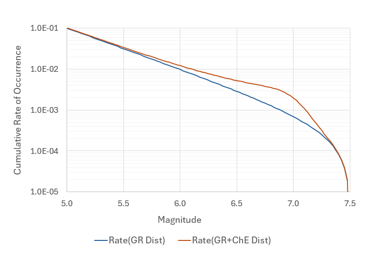
Figure 1. MRD for a hypothetical fault scenario with \(L=120\) km, \(W=12 \) km, and \(S=5\) mm/year with the occurrence rate of \(M \ge 5.0\) as 0.1. The GR distribution only releases about \(55\%\) of the accumulating seismic moment rate. The release of the leftover moment rate is formulated using a ChE model, red line.
It should be noted that the GR distribution is constructed using \(b=1.0\); see the link on GR distribution on the previous page for a more detailed discussion on the subject. The GR distribution in Figure 1 only releases about 55% of the total available seismic moment rate. The leftover seismic moment rate is released by a range of characteristic earthquakes, defined by a Gaussian distribution with a mean of \(M_{Ch}=7.0\) and \({\sigma}_M = 0.24\), only considering two standard deviations to capture the variation.
In practice, the upper bound magnitude for the GR distribution is often considered lower than the ChE upper bound magnitude. Figure 2 shows a different MRD for the fault scenario in Figure 1, using the GR upper bound magnitude of \(M=7.0\). The GR earthquakes in Figure 2 release only 30% of the total seismic moment rate. The rest is released by the characteristic earthquakes, which result in higher occurrence rates for large earthquakes than those shown in Figure 1.
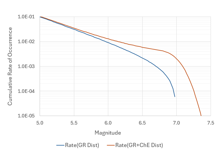
Figure 2. A plot of MRD for the fault scenario described in Figure 1, but using \(M=7.0\) as the GR upper bound magnitude. The Lower upper bound magnitude for GR, compared to that of Figure 1, is used to limit the magnitude overlap of GR and ChE distributions. The GR distribution releases about \(30\%\) of the total seismic moment. This results in higher rates of large-magnitude earthquakes than those in Figure 1.