Sand Box: Hazard Analysis for Earthquakes on Virtual Faults
In seismically active regions, buildings will experience different ground motions (GMs) intensities from earthquakes on different regional seismic sources. Seismic hazard analysis (SHA) quantifies the expected average annual frequencies for a site or building to experience ground motions higher than different assumed levels. Significant uncertainties exist in future earthquake occurrences, locations, magnitudes, and GMs. Given that, a robust SHA cannot be deterministic. All modern SHAs use probabilistic models to formulate the impacts of uncertainties on SHA. This is referred to as the probabilistic seismic hazard analysis (PSHA).
The likelihood that a site would experience a certain level of GM from any future earthquake in a complex way depends upon the tectonic setting of the region, the expected occurrence rates and spatial distribution of different magnitude earthquakes on different seismic sources, and the impacts of large-scale regional and local shallow site conditions on GMs, among other things. To conduct PSHA for a site, at the minimum, seismologists need to follow the following basic steps:
- Identify and delineate all seismic sources, including faults, subduction zones, and regions with random unknown sources.
- Quantify the magnitudes, rates of occurrences, mechanisms, and rupture geometries of all earthquakes on or within the identified sources
- Identify sets of ground motion prediction equations (GMPEs) relevant to the tectonic setting for estimating the expected GMs, i.e., the median (\(\mu\)) and standard deviation of the error (\(\sigma\)), for earthquakes given the rupture geometry, mechanisms, source-site distances, and shallow soil-site conditions
- For each site, calculate GMs intensities, i.e. \(\mu\) and \(\sigma\), for all earthquakes on different seismic sources to estimate the exceedance-probabilities of different GM levels (\(G_r\))
- For each site, calculate the exceedance rates of different \(G_r\) levels considering earthquakes occurrence rates and the \(G_r\) exceedance probabilities
- For each site, estimate the \(G_r\) exceedance rates using the calculated hazard from all earthquakes
- A hazard curve refers to a curve that represents the exceedance rates of various \(G_r\) levels at a site
Most PSHA only consider earthquakes of magnitude five and larger since the smaller magnitudes are not very damaging. Given any earthquake’s magnitude, source-site distance, and other source and site-related information, GMs parameters \(\mu\) and \(\sigma\) can be estimated using the identified regional GMPEs. Earthquake GMs follow lognormal distributions, i.e. \(ln(GM)\) follows a normal distribution. This is supported by years of GM recordings and theoretical formulation of earthquake GMs. Given an earthquake’s GM parameters, \(\mu\) and \(\sigma\), at a site, estimating the exceedance probabilities of different levels of GMs is straightforward. It should be noted that the median is defined as the expected value of \(ln(GM)\), and \(\sigma\) is the standard deviation for \(ln(GM)\) distribution.
Seismologists often formulate the occurrences of earthquakes as Poisson processes. A Poisson process assumes that the occurrences of earthquakes in time are independent. For any assumed magnitude range, there is a constant parameter (\(\lambda\)) that approximates the probability of occurrence of one or more events, the probability of more than one event is assumed to be negligible, in an infinitesimal time (\(\Delta t\)) interval as \(\lambda *\Delta t\). The parameter \(\lambda\) is typically interpreted as the average rate of occurrence. The Poisson process is often called a memory-less and time-independent process and plays an important role in formulating the time-independent PSHA. For an event with a Poisson distribution with an average rate of \(\lambda\), the probability of occurrence of one or more events within a time window \(T_w\) can be estimated as:
$$P=1-e^{-\lambda* T_w}…(1)$$
The following is a simple example of a PSHA analysis on a site. Suppose a region has experienced five earthquakes of \(M \approx 6.0\) within the last 100 years. This translates to the annual rate of occurrence of \(5/100 = 0.05\). Using this info, one can easily estimate the expected exceedance rates for GMs corresponding to, say, \(\mu\) and \(\mu + \sigma\). The exceedance probabilities of \(ln(GM)\) for these GM levels from the lognormal distribution are estimated as 50% and 16%, respectively. Given the expected annual occurrence rate for \(M \approx 6.0\), the exceedance rate for \(\mu\) and \(\mu + \sigma\) levels are estimated as 0.05*0.50= 0.0025 and 0.05*0.16 = 0.008, respectively. The exceedance probabilities in 30 years are estimated as \(1-e^{-0.025*30} = 0.53\), i.e. \(53\%\) and \(1-e^{-0.008*30} = 0.21\), i.e. \(21\%\), respectively, see equation 1.
It is worth mentioning that in this example, assuming a Poisson process for earthquake occurrences, the probability of experiencing one or more earthquakes of \(M \approx 6.0\) within a 30-year time window is estimated as \(1-e^{-0.05*30} = 0.78\), i.e., \(78\%\).
The following schematic diagram demonstrates a typical PSHA for three virtual faults.
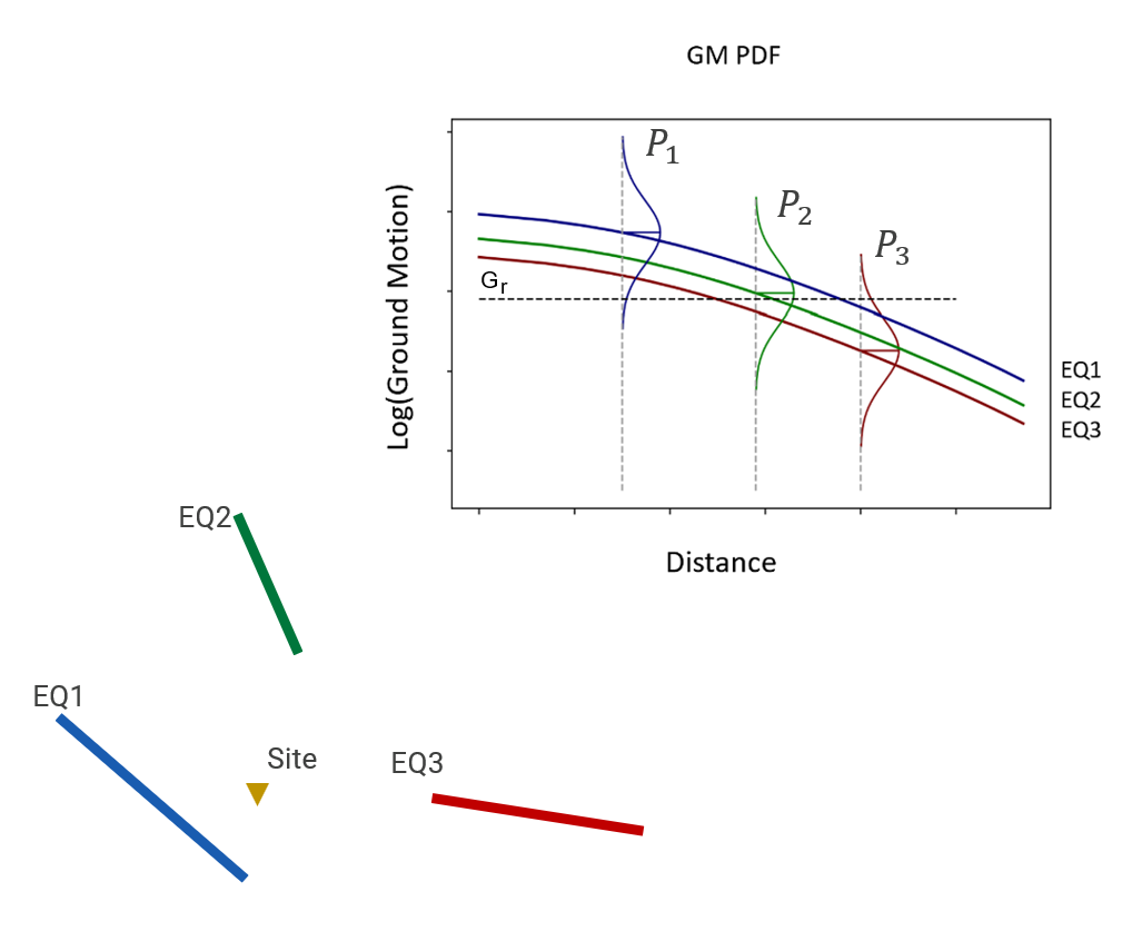
Figure 1. A schematic diagram of three faults and their GM estimates at a site. The \(G_r\) exceedance probability for each earthquake is the area under the lognormal distribution curve above the \(G_r\) level.
Let’s assume the faults are capable of causing earthquakes of magnitudes \(M_1\), \(M_2\), \(M_3\) with the annual rates of \(\lambda_1\), \(\lambda_2\), and \(\lambda_3\), and GMs that are represented by lognormal distributions, i.e. normal distribution in a log scale.
For each earthquake, the rate of exceedance of any assumed reference ground motion \(G_r\), see Figure 1, can be calculated as the product of \(G_r\)-exceedance probability, the area under the GM distribution above \(G_r\) level, and the occurrence rate of the earthquake. The total annual exceedance rate for \(G_r\) is calculated as
$$R_e=\lambda_1*P_1+\lambda_2*P_2+\lambda_3*P_3…(2)$$
The exceedance probability of \(G_r\) within a time window \(T_w\) is estimated as
$$P_e=1-e^{-R_e*T_w}…(3)$$
To demonstrate a typical analysis, let’s assume \(\lambda_1=0.001\), \(\lambda_2=0.01\), and \(\lambda_3=0.004\). As was discussed earlier, \(ln(GM)\) follows a normal distribution. The exceedance probability of \(G_r\) can be estimated by mapping \(G_r\) to an equivalent Z-score for normal distribution and using the standard probability table to calculate the corresponding exceedance probability.
$$Z_{G_r}=\frac {ln(G_r)-\mu}{\sigma}…(4)$$
where \(\mu\) and \(\sigma\) are the median and standard deviation of error of \(ln(GM)\).
Let’s assume that for our schematic diagram example, we calculate Z = -2.5, -0.2, and 2 for the three earthquakes. Using the cumulative probability table for the normal distribution, the three Z-scores translate to 99.4%, 57.9%, and 2.3% exceedance probability for \(G_r\) from the three earthquakes. The overall exceedance rate is calculated as follows:
$$R_e=0.001*0.9938+0.01*0.5793+0.004*0.0228 = 0.00688…(5)$$
The \(G_r\) exceedance probabilities within 10, 30, and 50 years are be calculated as
$$P_{10}=100*(1-e^{-0.00688*10}) \approx 6.6\%…(6)$$
$$P_{30}=100*(1-e^{-0.00688*30}) \approx 18.6\%…(7)$$
$$P_{50}=100*(1-e^{-0.00688*50}) \approx 29.1\%…(8)$$
In a real full-scale hazard analysis scheme, a site is exposed to hazards from thousands of earthquakes on known faults and unknown random sources. The PSHA should also consider the uncertainties in magnitude-rate, spatial, and geometrical distributions of earthquakes, earthquake source mechanisms, ground motion calculations, and shallow soil conditions.
For engineering design and risk mitigation purposes, it is required to estimate regional or site-specific GM values that correspond to specific hazard and risk criteria. To be able to assess the GM values corresponding to the design risk values at sites of interest, it is the common practice to calculate exceedance rates for a large range of \(G_r\) values with fine sampling interval, typically at 0.01 g, at sites and use the results to extrapolate for GM values that correspond to the required risk criteria. For example, an engineer might need to know the expected GM at the project site with \(10\%\), \(2\%\), and/or \(1\%\) probability of exceedance in 50 years. Using the Poisson probability formulation, the corresponding annual exceedance rates are calculated as follows:
$$\lambda_{10\%} =-ln(1 – 0.10)/50 =0.0021…(9)$$
$$\lambda_{2\%} =-ln(1 – 0.02)/50 =0.0004…(10)$$
$$\lambda_{1\%} =-ln(1 – 0.01)/50 =0.0002…(11)$$
As discussed earlier, the GM values corresponding to these exceedance rates can be easily estimated using the calculated exceedance-rate GM database for the site. Figure 2 shows a typical hazard map for the US, published by the United States Geological Survey (USGS), for peak ground acceleration (PGA) with 2% PE in 50 years. The core of PSHA used to create this map is discussed here.
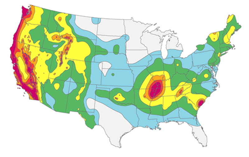
Figure 2. USGS hazard map of PGA with \(2\%\) probability of exceedance in 50 years