Decades of research have produced methodologies for interpreting regional rates of surface strain‑rate measurements in terms of regional rates of seismic moment accumulation. Because seismic moment quantifies the strain released by earthquakes, framing regional strain buildup in terms of moment rate offers a meaningful way to assess the potential for future seismic activity.
In this context, the geodetic seismic moment rate is typically formulated as:
$$\dot{M}_{geod}=2*\mu*A*H*\dot{\epsilon}…(1)$$
where \(\dot{M}_{geod} \) is the geodetic moment rate, \( \mu\) is shear modulus, \(A\) is the area, \(H\) is the seismogenic depth that is experiencing strain, and \( \dot{\epsilon}\) is a practical measure of surface strain that is most suitable for estimating \(\dot{M}_{geod} \).
The proper choice of \( \dot{\epsilon}\) in equation 1 is a challenge. Kostrov (1974), Savage and Burford (1973), Savage (1983), Anderson (1979), Ward (1994, 1998a, 1998b), and the Working Group on California Earthquake Probabilities (1995) have all tackled this issue and recommended choices for \(\dot{\epsilon}\). To better understand the formulation of \( \dot{\epsilon}\), we have to review a few of the strain terminology from engineering mechanics.
The principal strain components for a 2D strain measurement can be formulated as
$$\epsilon_{max}, \epsilon_{min}=\frac{(\epsilon_{xx}+\epsilon_{yy})}{2} + \sqrt{ {\frac{ (\epsilon_{xx}-\epsilon_{yy}) } {2} }^2+{(\epsilon_{xy})}^2}…(2) $$
The strain invariants are formulated as
$$I_1 = \varepsilon_{xx} + \varepsilon_{yy}…(3) $$
$$I_2 = \epsilon_{xx} \epsilon_{yy} – \gamma_{xy}^2…(4) $$
where \(\gamma_{xy} = 2*\epsilon_{xy}\). \(I_1\) mostly represents the volumetric change and \(I_2\) captures the effects of both normal and shear strains. Using the invariants, the principal 2D strain values can be estimated as the roots of the following equation.
$$\epsilon^2 – I_1 \epsilon + I_2 = 0…(5)$$
The UNAVCO and GEM strain rate maps, Figures 1, 2, and 3, are constructed using the second invariant, \(I_2\). The following are a few of the recommendations you might find in the literature:
$$ \dot{\epsilon}={\epsilon}_{min}…(6)$$
$$ \dot{\epsilon}= \dot{\epsilon}_{max} – \dot{\epsilon}_{min}…(7)$$
$$ \dot{\epsilon}=Max(| \dot{\epsilon}_{max}|, | \dot{\epsilon}_{min}|)…(8) $$
$$ \dot{\epsilon}=Max(| \dot{\epsilon}_{max}|, | \dot{\epsilon}_{min}|,| \dot{\epsilon}_{max}+ \dot{\epsilon}_{min}|)…(9) $$
These different measures of strain rates certainly add to the inherent uncertainty when using geodetic data for developing regional seismicity. However, studies conducted by various researchers suggest that the level of uncertainty, due to different choices of \( \dot{\epsilon} \), is not very large, approximately 20%. However, it is universally recommended that modelers compare \(\dot{M}_{geod} \), \(\dot{M}_{geol} \), and \(\dot{M}_{seis} \) to evaluate the integrity of these different data types before integrating the information to construct regional seismic models.
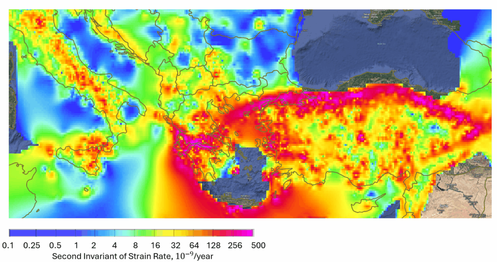
Figure 1.
Figure 2.
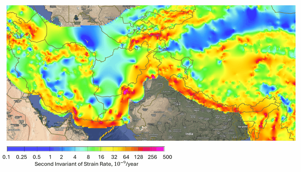
Figure 3